


- Monetary Policy
- Economic
- Economics
- History
This article appeared in the Wall Street Journal the day after Milton Friedman’s death. He adapted it from an academic paper on which—at the age of 94—he had been working.
The third of three episodes in a major natural experiment in monetary policy that started more than 80 years ago is just now coming to an end. The experiment consists in observing the effect on the economy and the stock market of the monetary policies followed during, and after, three very similar periods of rapid economic growth in response to rapid technological change: to wit, the booms of the 1920s in the United States, the 1980s in Japan, and the 1990s in the United States.
The prosperous 1920s in the United States were followed by the most severe economic contraction in its history. In our Monetary History (1963), Anna Schwartz and I attributed the severity of the contraction to a monetary policy that permitted the quantity of money to decline by one-third from 1929 to 1933. Since 1963, two episodes have occurred that are almost mirror images of the U.S. economy in the 1920s: the 1980s in Japan, and the 1990s in the United States. All three episodes were marked by a long period of rapid economic growth, sparked by rapid technological change and the emergence of new industries, and accompanied by a stock market boom that terminated in a crash. Monetary policy played a role in these booms but only a supporting role. Technological change appears to have been the major player.
These three episodes provide the equivalent of a controlled experiment to test our hypothesis about what we termed the Great Contraction. In this experiment, the quantity of money is the counterpart of the experimenter’s input. The performance of the economy and the level of the stock market are the counterpart of the experimenter’s output, that is, the variables whose relation to input the experimenter is seeking to determine. The three boom episodes all occurred in developed private enterprise market economies involved in international finance and trade and with similar monetary systems, including a central bank with power to control the quantity of money. This is the counterpart of the controlled conditions of the experimenter’s laboratory.
The Money Supply
In addition, history has provided a close counterpart to the kind of variation in input that our hypothetical experimenter might have deliberately chosen. Monetary policy, as measured by the behavior of the quantity of money, was very similar in the three boom periods and very different in the three post-boom periods, with settings that might be described as low, medium, and high (see figure 1).
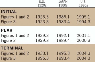
To measure the quantity of money, I use M2 in the United States and the conceptually equivalent M2 plus certificates of deposit in Japan. To express the data for the two countries and the widely separated periods in comparable units, I use as an index of the money stock the ratio of the quantity of money to its average value for the six years prior to the cycle peak. The peak quarter of the relevant business cycle is the third quarter of 1929 (29.3) for the earlier U.S. episode; the first quarter of 1992 (92.1) for Japan; and the first quarter of 2001 (01.1) for the second U.S. episode (see table 1). Finally, the data are plotted to align the dates at the cycle peak.
For the striking contrast between the period before the cycle peak and the period after the cycle peak, see figure 1. There are some differences before the peak—money growth is slowest on the average for the earlier U.S. episode, fastest for Japan—but the differences are small; there is reasonably steady money growth in all three episodes. The contrast with the period after the cycle peak could hardly be greater. Money supply declines sharply after the cycle peak in the first episode, goes from stable to rising mildly in the second, and rises steadily and sharply in the third. Our hypothetical experimenter planned his experiment well.
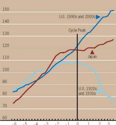
The GDP
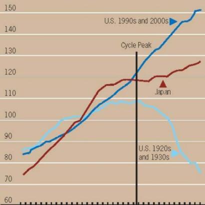
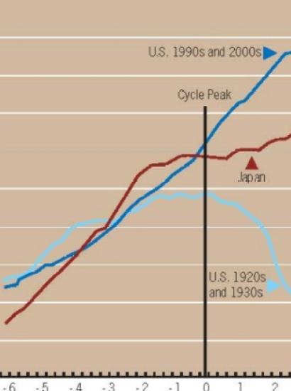
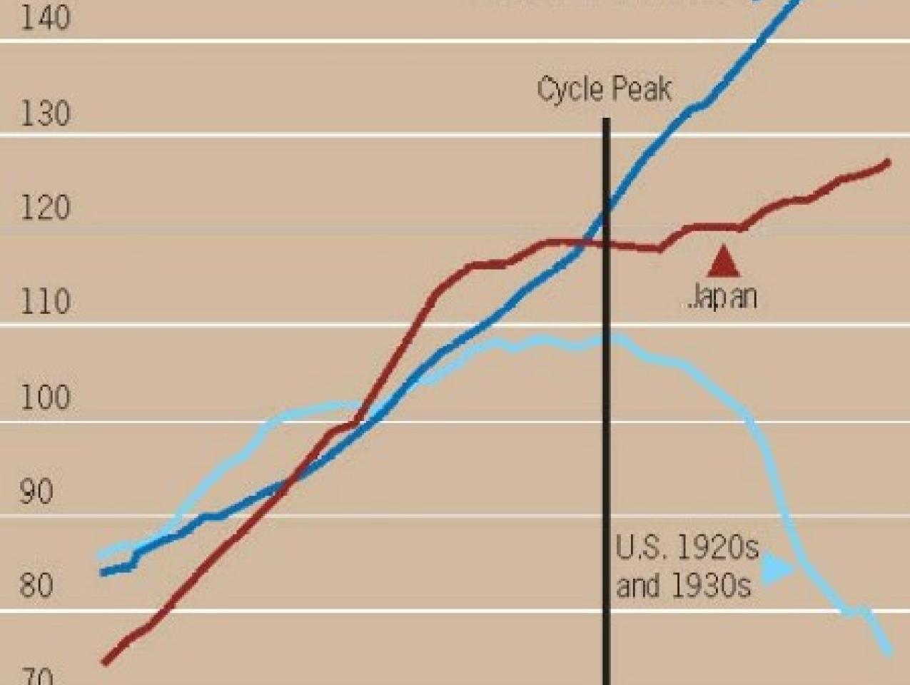
The results of the third episode of this natural experiment are now all in. To see how GDP in nominal terms (dollars or yen in current prices) behaved during the boom and post-boom periods, see figure 2. I use nominal GDP rather than real GDP because M2 is also a nominal magnitude. How changes in nominal GDP are divided between prices and output is an important question but one that is not directly relevant to this experiment. One further preliminary comment: I believe the erratic behavior of nominal GNP during the 1920s and 1930s is largely a statistical artifact. The data for that period are scarce and of poor quality.
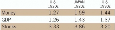
As figure 1 shows, there is a striking contrast between the boom and the post-boom periods: roughly similar growth during the booms, widely variable growth during the post-boom. Both before and after the cycle peak, nominal GDP growth paralleled monetary growth. During the boom, money and nominal GDP grew most rapidly in Japan, most slowly in the first U.S. episode, and at an intermediate rate in the second U.S. episode. The ratio of the money stock at the cycle peak to its value six years earlier (the initial date in the figures) and the corresponding ratio for GDP are seen in table 2. In the first two rows of the table, the ratios are highest for Japan, lowest for the United States in the 1920s.
After the cycle peak, money fell sharply in the first episode and so did nominal GDP; money growth stagnated in the second episode and so did GDP; money grew at a rapid rate in the third episode and, after a brief lag (corresponding to the mild 2001 recession), so did GDP. The ratio of the money stock at the terminal date plotted to its value at the cyclical peak and the corresponding ratio for GDP is seen in table 3. Both ratios are decidedly lowest for the U.S. 1920s, and decidedly highest for the U.S. 1990s.
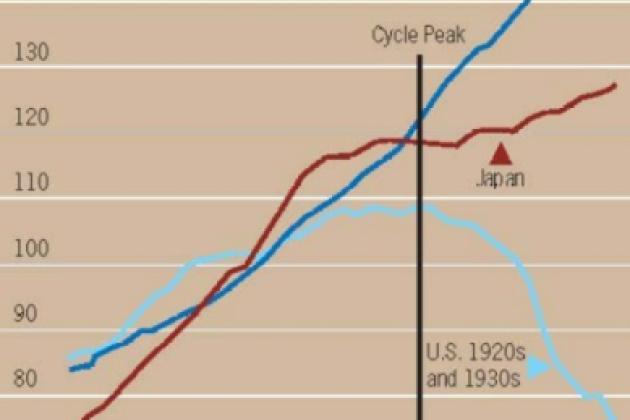
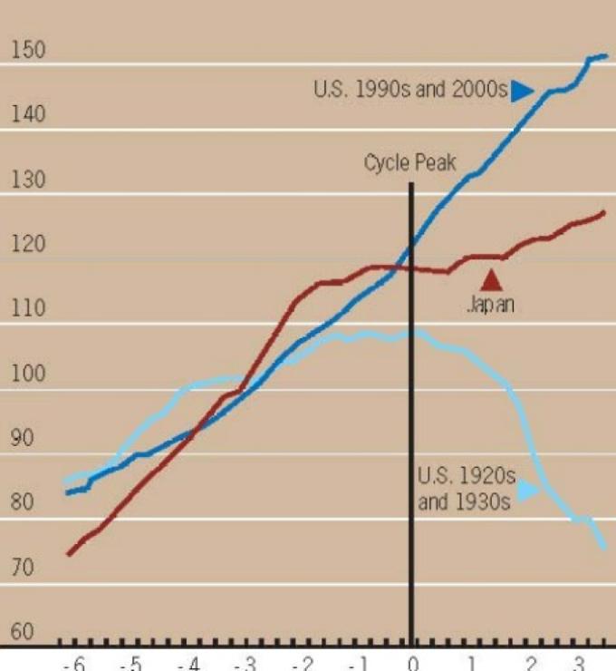
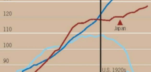
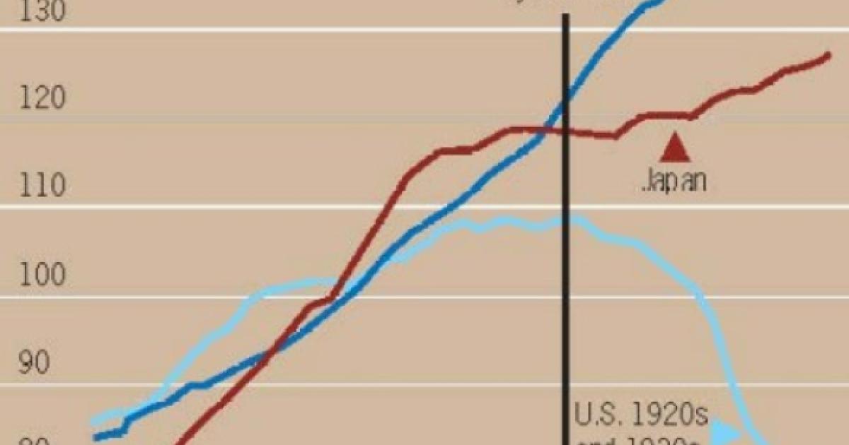
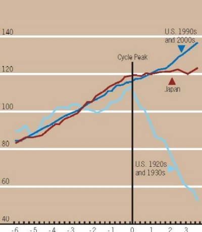
The Stock Market
The peak of the stock market, as measured by the S&P index, coincided with the cycle peak in the first episode, both occurring in the third quarter of 1929 (29.3). That was not the case, however, in the later episodes. In Japan, stock prices as measured by the Nikkei peaked in the fourth quarter of 1989 (89.4), nine quarters before the cycle peak. In the second U.S. episode, stock prices as measured by the S&P 500 peaked in the third quarter of 2000 (00.3), two quarters prior to the cycle peak. (See figure 3, which plots the data to align the series at the stock market peak.)
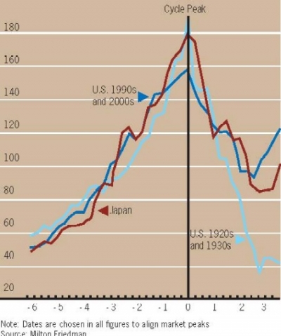
The near identity of the three stock market series during the boom is truly remarkable. Yet even the minor deviations that exist reflect to some extent the differences in monetary growth, as table 2 makes clear. Money growth was highest in Japan, and the Nikkei shows the largest rise in the stock market. The other two do not conform: money rose more in the 1990s than in the 1920s, whereas stock prices rose slightly less; see the ratio of peak to initial value in table 2.
Of more interest for our purpose is what happened after the peak. For the following year, the three stock price series fell in tandem, responding to the inner dynamics of a collapsing bubble. Then, the differences in monetary policy began to have an effect. Beginning in late 1930, the S&P index started falling away from the others under the influence of a collapsing money stock. For another year and a half, the other two indexes move in tandem. Then the much more expansive policy of the Fed in the 1990s than that of the Bank of Japan in the 1980s takes effect and pulls the S&P 500 away from the Nikkei, which stabilizes in response to the passive monetary policy of the Bank of Japan (see table 3).
The results of this natural experiment are clear, at least for major ups and downs: What happens to the quantity of money has a determinative effect on what happens to national income and to stock prices. The results strongly support Anna Schwartz’s and my 1963 conjecture about the role of monetary policy in the Great Contraction. They also support the view that monetary policy deserves much credit for the mildness of the recession that followed the collapse of the U.S. boom in late 2000.